We begin by simulating survey data for two commensal species for the following scenario. Species 1 has a 50% probability occupancy. Species 2 benefits from the presence of species 1, so its probability of occupancy is 83% when species 1 is also present, but only 50% in the absence of species 1. One hundred sites are surveyed 10 times each. The probability of detection for both species is 0.3.

data_generator_commensal_species = function(psi, p, nSites, nReps){ # occupancy prob psi, detection prob p
 # true occupancy state
 z1 <- rbinom(nSites, 1, psi)
 z2 <- rbinom(nSites, 1, psi + z1/3)
 # sampling of true occupancy state
 y1 <- matrix(NA, nSites, nReps)
 y2 <- matrix(NA, nSites, nReps)
 for(i in 1:nSites) {
 y1[i,] <- rbinom(nReps, 1, z1[i]*p) # detection history for species 1
 y2[i,] <- rbinom(nReps, 1, z2[i]*p) # "" species 2
 }
 list(y1,y2)}
y = data_generator_commensal_species(psi = .5, p = .3, nSites = 100, nReps = 10)

We specify the model structure in jags.

model {
## Priors
a0 ~ dunif(-5, 5)
b0 ~ dunif(-5, 5)
b1 ~ dunif(-5, 5)
p ~ dunif(0, 1)

## Model
# State process
for(i in 1:nSites) {
 logit(psi1[i]) <- a0
 logit(psi2[i]) <- b0 + b1 * Z1[i]
 Z1[i] ~ dbern(psi1[i])
 Z2[i] ~ dbern(psi2[i])
# Detection process
 for(j in 1:nOccs) {
   y1[i, j] ~ dbin(p, Z1[i])
   y2[i, j] ~ dbin(p, Z2[i])
   }
 }
}

Then we fit the model with R and jags.

library(rjags)
d = list( y1 = y[[1]], y2 = y[[2]], nSites = 100, nOccs = 10)
mod = jags.model("commensal_multispecies.txt", d)
update(mod)
post = coda.samples(mod, c("a0", "b0", "b1", "p"),1e4)
summary(post)
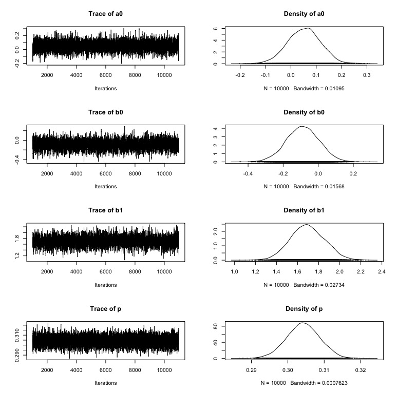
plot(post)

Here are the posterior distributions. A nice fit to the scenario for the simulated data.